Cavity flows have been the subject of aerodynamic research since the early days of high-speed aircraft with internal store carriage in the 1950s. Low observability design requirements for current combat aircraft has renewed the interest in this field. The presence of an open cavity, such as a weapon or undercarriage bay, exposed to a high-speed grazing flow can result in severe pressure fluctuations. These pressure fluctuations can reach intensities of up to 165dB SPL and may cause damage to both the aircraft and to any sensitive components within the bay. Results for this study were generated using an existing generic rectangular planform cavity wind tunnel model, designated as M219/1. This small scale model was the forerunner for the more widely known larger scale M219 generic cavity model.
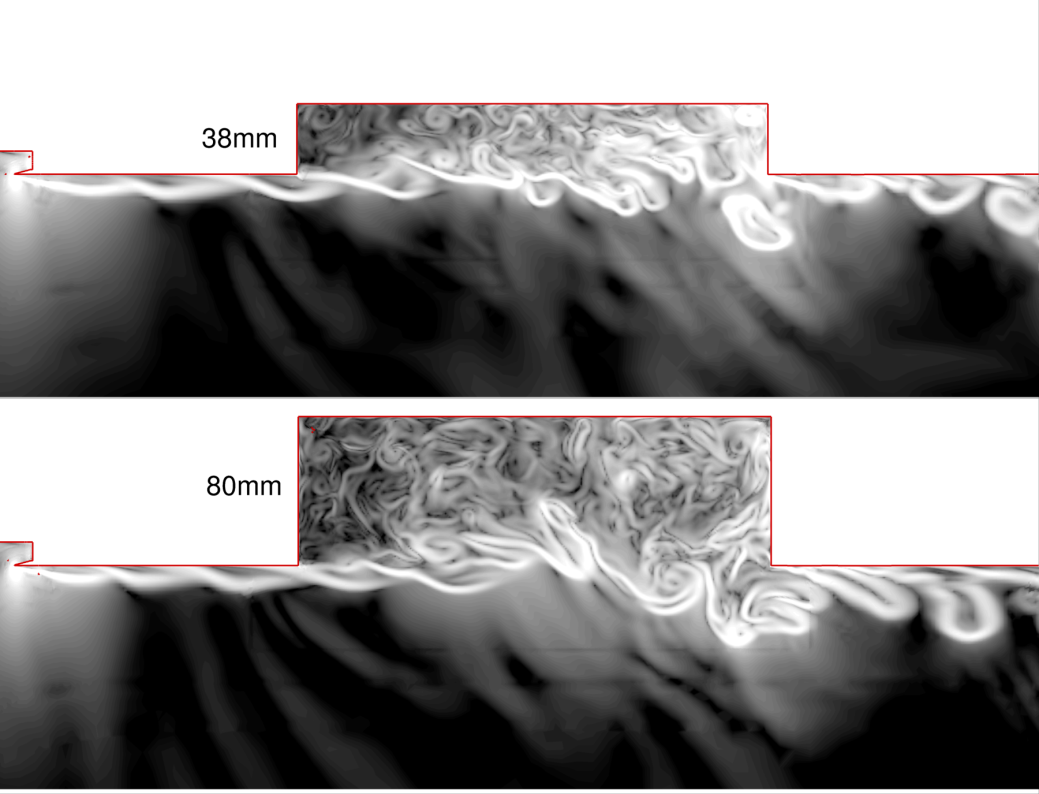
Numerical simulations were performed for two geometries, the 38mm and 80mm deep cavities, at a freestream Mach number of 0.80. In order to capture the unsteady flow behaviour in the cavity, a time accurate detached eddy simulation (DES) model was run which uses Reynolds averaged Navier-Stokes (RANS) near to the wall to reduce computational cost and a large eddy simulation (LES) model in the separated flow region far from the walls.
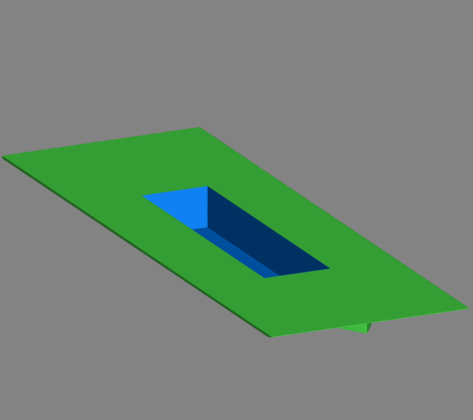
The geometry modelled in the numerical simulations is shown to the far left. The splitter plate and plinth geometry were included in the calculations as the boundaries of the plate are close to the cavity edges – this is often excluded from this type of calculation. The wind tunnel walls were not included in the model because there was no affordable way to model the perforated walls in the CFD code. The effect of the walls is not known. The rectangular far-field boundary extends 6 meters (23l) up and downstream of the cavity and 5 meters (19l) on each side.
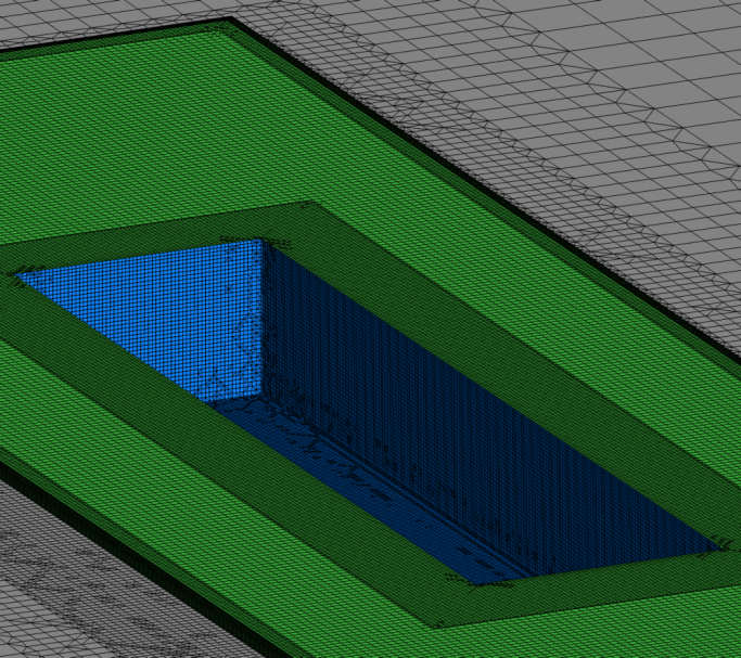
Unstructured, hex-dominant and prism layer meshes were generated for both cases using the BoxerMesh software. The mesh for the 38mm cavity is shown in above (right image). Inside the cavity the mesh is isotropic with a spacing of Δx=1mm giving l/Δx=254. This results in mesh sizes of 12 and 14 million cells for the two geometries. Adiabatic wall boundary conditions were applied to all solid surfaces and a Riemann far-field boundary condition was used to represent the freestream flow at the wind tunnel conditions.
A time-step of Δt=3× 10⁻⁶s was used in order to give a CFL number of approximately 1 in the isotropic cells in the cavity. The Cobalt was initially run for 5000 time steps to allow the flow to establish itself and to flush out any transients and then data was recorded for 100,000 time steps giving a sample length of 0.3s. Data was recorded every 8 steps giving 12500 samples. Data was sampled at the transducer locations and in a grid of 75×300 points on the cavity ceiling to compare with the DPSP results.
The data was processed using a Fast-Fourier Transform method, which was then scaled accordingly to Power-Spectral Density (PSD). The process was conducted with a sample size of 2048 and a 50% overlap, which, allows an ensemble average of 11 data blocks and gives a frequency resolution of approximately δf=20Hz.
| Case | Mesh | Turb Model | Mach | pinf (Pa) | Tinf (K) | Δt |
| 1 | 38mm | DES-SA | 0.8 | 65696.7 | 244.4 | 3×10⁻⁶ |
| 2 | 80mm | DES-SA | 0.8 | 65696.7 | 244.4 | 3×10⁻⁶ |
Table 3: CFD Cases Run
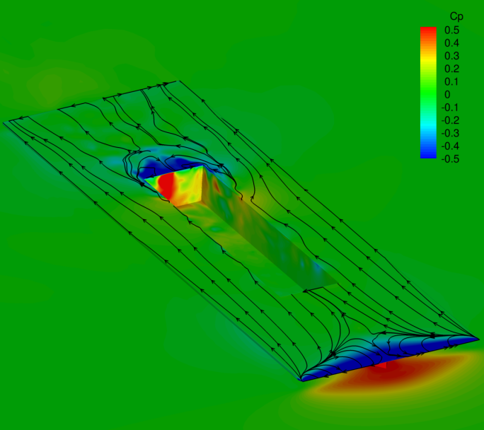
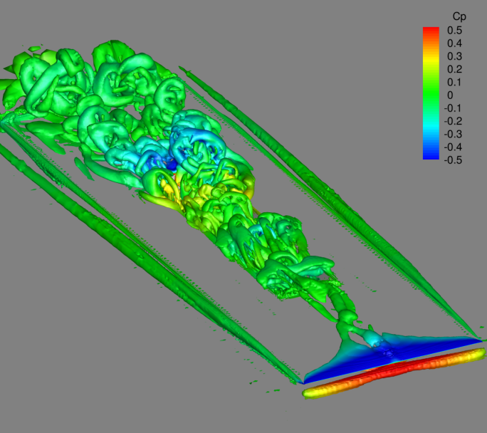
Flowfield visualisation of the instantaneous numerical results (shown immediately below) reveals that the flow at the leading edge of the cavity rig may not be attached or steady as was probably the intention with the design of this rig. The wedge shaped leading edge of the splitter plate causes the flow to separate on the upper surface, reattaching some distance downstream. The presence of this separation means the boundary layer approaching the cavity cannot be predicted using approximation formulae for boundary layer thickness and is probably much thicker than anticipated. The separation is also unsteady and causes vortex shedding that flows over the cavity. This can be seen in the q-criterion plot (below, right) and in the centreline slices shown further below. Despite these unexpected features, the setup should match what was tested in the wind tunnel and therefore the agreement should be much better than for a flat plate numerical model. This experience illustrates how useful prior information from numerical simulations can be for designing representative models or better understanding any spurious results from experiments.
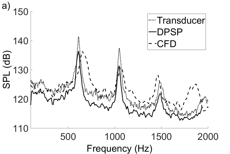
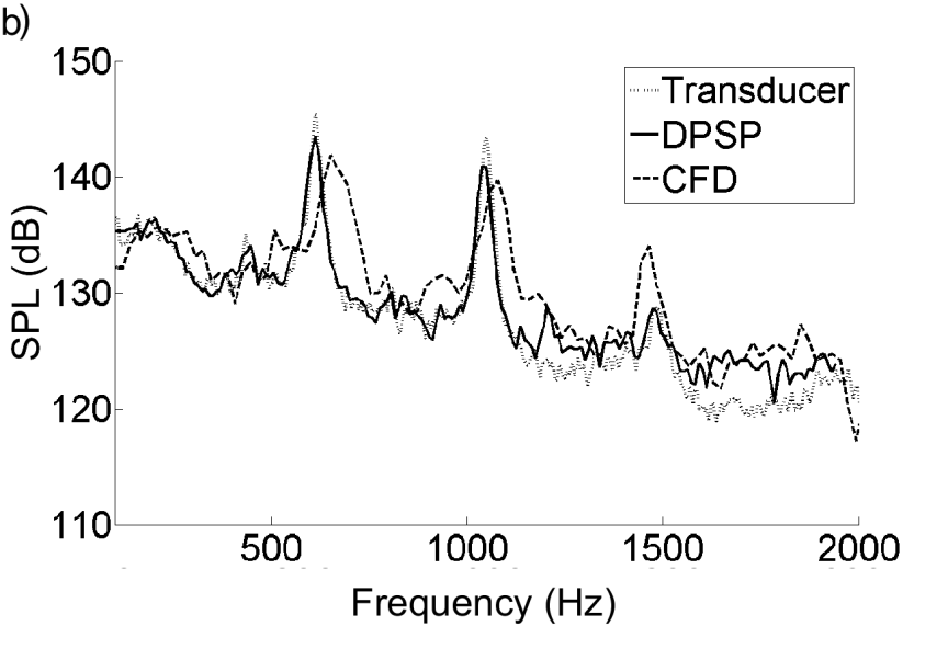
 The cavity ceiling was instrumented along its centreline with 5 unsteady pressure transducers (Kulite XCS-190M-15A) at fractional cavity lengths (x/l) of 0.1, 0.3, 0.5, 0.7, and 0.9. The tunnel static pressure (P) was measured from a static pressure tapping located on the tunnel floor at a location corresponding to a cavity fractional length of x/l=0.1. The tunnel total pressure (P0) was measured using a Pitot probe located upstream within the settling chamber of the tunnel and it was assumed that there would be no loss in total pressure between the measurement location and working section. Both tunnel pressures (P and P0) were measured using Druck 15psi differential transducers.The numerical results for the datum case (l/h=6.7) also match the measured data fairly well. Broadband noise levels are calculated to be within 1dB of the measured levels, with peak tonal magnitudes to within 4dB. The numerical results predict modal frequencies which are within 3% of those measured by the transducers (see below). The differences between the measured and predicted sound pressure levels and numerical frequencies may be due to difficulties in modelling the flowfield over the splitter plate.
For more detailed information, you can read the full paper: Evaluation of Dynamic Pressure-Sensitive Paint for Improved Analysis of Cavity Flows and CFD Validation